Mueez Khan
Mueez Khan

Generating Plotly charts for water data with Python and Polars
Explore an interactive walkthrough of how to generate Plotly charts about water data from Boerne Utilities using Python and Polars.
Published: 2025-12-12
Last updated: 2025-12-15
work
python
plotly
polars
"The dashboard was created to support water management decisions by individuals, communities, and utilities to promote better stewardship of water resources and greater resilience during droughts or water supply challenges." — Boerne UtilitiesIt wasn't only the web app that was new, rather I also recalculated the data necessary to render each of the , , and on the web app.
Why I used Rust for the dashboard's data processing







Why I am using Python for this blog post
Rather than showing , the purpose of the rest of this post is to showcase what overall calculations were made using Polars on the water utility data for generating the visualization of the daily total water demand chart. I'll attempt to showcase how to get from the raw data to an interactive data visualization. Therefore I'll be using Python and Polars. You may also find this post useful as a demonstration of the Python Polars library. Since we're focusing on the data processing, I also won't reproduce the exact same visualization as the one on the Boerne Water Data Dashboard (as that would also be too time-consuming).ETL process demonstration for total daily water demand
If you're on a mobile device then for the rest of this post (or at least for the tables and chart) you may want to rotate your phone to landscape mode .
Much of the rest of this post is based on a Jupyter Notebook and assumes you're familiar with local Python development/analysis.Loading the water utility data
Most of the water utility data is provided as a spreadsheet by the utilities director. We have a re-uploaded CSV file we can download and use for demonstrating some of the primary calculations used to generate theDaily total water demand chart on the Boerne Water Data Dashboard.
We'll download the latest water utility data from boernetx.thewaterdata.com/data/utility-data.csv.
After downloading the data, we'll install polars, plotly, and numpy by running the following:
pip install polars plotly numpyimport polars as pl
df = pl.read_csv("utility-data.csv")
df.head()| Date | City Wells | Boerne City Lake | GBRA Total | GBRA Del. To KW | Canyon Lake (GBRA) | Reclaimed Water (WWTRC) | Total Water Demand | Water Treatment Plant Rainfall | City of Boerne Population | City Water Utility Service Population | Reclaimed Water Service Poulation |
| 5/19/2000 | 373 | 382 | 755 | ||||||||
| 5/20/2000 | 326 | 527 | 853 | ||||||||
| 5/21/2000 | 347 | 554 | 901 | ||||||||
| 5/22/2000 | 473 | 398 | 871 | ||||||||
| 5/23/2000 | 564 | 553 | 1,117 |
Casting the Date column from str to date
Let's turn the Date column's datatype from str to date so we can perform operations on the data.
df = df.with_columns(
    pl.col("Date").str.to_date("%m/%d/%Y")
)

df.head()| Date | City Wells | Boerne City Lake | GBRA Total | GBRA Del. To KW | Canyon Lake (GBRA) | Reclaimed Water (WWTRC) | Total Water Demand | Water Treatment Plant Rainfall | City of Boerne Population | City Water Utility Service Population | Reclaimed Water Service Poulation |
| 2000-05-19 | 373 | 382 | 755 | ||||||||
| 2000-05-20 | 326 | 527 | 853 | ||||||||
| 2000-05-21 | 347 | 554 | 901 | ||||||||
| 2000-05-22 | 473 | 398 | 871 | ||||||||
| 2000-05-23 | 564 | 553 | 1,117 |
Date column to have a data type of date, so we can perform certain date-related operations on the dataframe using Polars.
Implementation insight
For the actual implementation used for the Boerne Water Data Dashboard, we also run a filter for values from the most recent year(s) since it's not necessary to recalculate demand data for more historic records on each run.
Representing the Total Water Demand column in Millions of Gallons per Day (MGD)
For the Total Water Demand column we'll want to perform the following:
- Remove commas by replacing them with an empty string
- Cast the column from
strtof64(e.g. decimal numbers) - Divide the values by
1000 - Round to
6digits
df = df.with_columns(
    (pl.col("Total Water Demand").str.replace_all(",", "", literal=True).cast(pl.Float64) / 1000).round(6)
)

df.head()| Date | City Wells | Boerne City Lake | GBRA Total | GBRA Del. To KW | Canyon Lake (GBRA) | Reclaimed Water (WWTRC) | Total Water Demand | Water Treatment Plant Rainfall | City of Boerne Population | City Water Utility Service Population | Reclaimed Water Service Poulation |
| 2000-05-19 | 373 | 382 | 0.755 | ||||||||
| 2000-05-20 | 326 | 527 | 0.853 | ||||||||
| 2000-05-21 | 347 | 554 | 0.901 | ||||||||
| 2000-05-22 | 473 | 398 | 0.871 | ||||||||
| 2000-05-23 | 564 | 553 | 1.117 |
Selecting relevant columns for the visualization
We'll want to select the relevant columns from the original data for our visualization. These include theDate and Total Water Demand columns.
df = df.select(
    [
        pl.col("Date"),
        pl.col("Total Water Demand")
    ]
)

df.head()| Date | Total Water Demand |
| 2000-05-19 | 0.755 |
| 2000-05-20 | 0.853 |
| 2000-05-21 | 0.901 |
| 2000-05-22 | 0.871 |
| 2000-05-23 | 1.117 |
Preparing dataframe for multiple chart visualizations
We'll be generating several visualizations, one for each year. Therefore it would also be helpful to add two columns to our dataframe:Year(e.g.2025) - for partitioning the dataframe by yearMonth and day(e.g.Jan-01) - for the x-axis in each visualization
df = df.with_columns(
    pl.col("Date").dt.year().alias("Year")
).with_columns(
    pl.col("Date").dt.strftime("%b-%d").alias("Month and day")
)

df.head()| Date | Total Water Demand | Year | Month and day |
| 2000-05-19 | 0.755 | 2000 | May-19 |
| 2000-05-20 | 0.853 | 2000 | May-20 |
| 2000-05-21 | 0.901 | 2000 | May-21 |
| 2000-05-22 | 0.871 | 2000 | May-22 |
| 2000-05-23 | 1.117 | 2000 | May-23 |
Implementation insight
Note that in the actual implementation we add another step to add a row of null data with the date February 29 on non-leap years for the plot to render properly. If the year has data past Feb 28 and there is no row for Feb 29 (non-leap years) then we add a Feb 29 entry with a null Total Water Demand value (allows for proper Plotly chart render when overlaying years).
Partitioning the dataframe by year
Now we can partition the dataframe by theYear column to get several dataframes, one for each year.
dfs = df.partition_by("Year")Generating visualizations for each year as interactive scatter plots with Plotly express
Finally we can iterate over each dataframe in our dataframes arraydfs and view them as an interactive visualization using the Plotly express library.
import plotly.express as px

for curr_df in dfs:
    year = curr_df.item(0, "Year")
    px.scatter(
        curr_df,
        x="Month and day",
        y="Total Water Demand",
        title=f"Daily Total Water Demand (MGD) in {year}",
    ).show()
print("")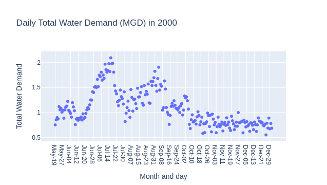 There are many other changes and steps involved to get to the visualization displayed on the Boerne Water Data Dashboard. However we have fulfilled the purpose of demonstrating how to get from the water utility data to a rudimentary interactive visualization.
Implementation insight
In the actual implementation I used the Rust Polars library to extract, transform, and load the data while using the react-plotly.js library with Next.js to organize interactive charts on the water data dashboard.
Explore the live chart
You can explore the finalDaily total water demand chart embedded below.
Conclusion
Combining Polars with visualization libraries such as Plotly can help resolve real-world issues such as water resiliency in Boerne, Texas. Hopefully this demonstration with Python helped you understand what kind of computations can be used to transform raw data and generate an interactive visualization to inform "individuals, communities, and utilities". Feel free to learn more about the dashboard or share your thoughts below.Changelog
Updates made to this blog post over time.
- Added animated underlines for the selected column headers in the "Selecting relevant columns for the visualization" section.
- Change "We now have" to "We have now".
Share your thoughts
Submit a comment about this post that may be shared.
Join the Newsletter
Receive updates during my career.
Featured Publications
Technical writing on work experiences, projects, and tools you may find useful.
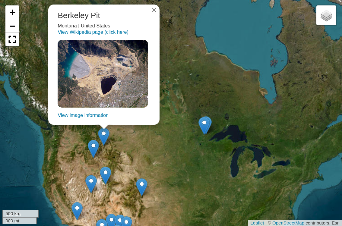
Mapping open-pit mines in the US
Python
Polars
Folium
Leaflet
Marimo
New "Typing with Typst" course

Typst
Generating Plotly charts for water data
Python
Polars
Plotly
Data visualization
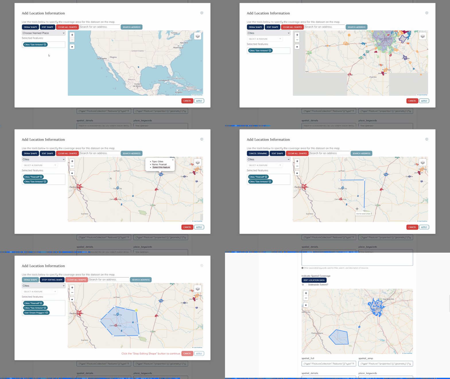
Gazetteers for Texas Water Data Hub
JavaScript
HTML/CSS
Python
Leaflet
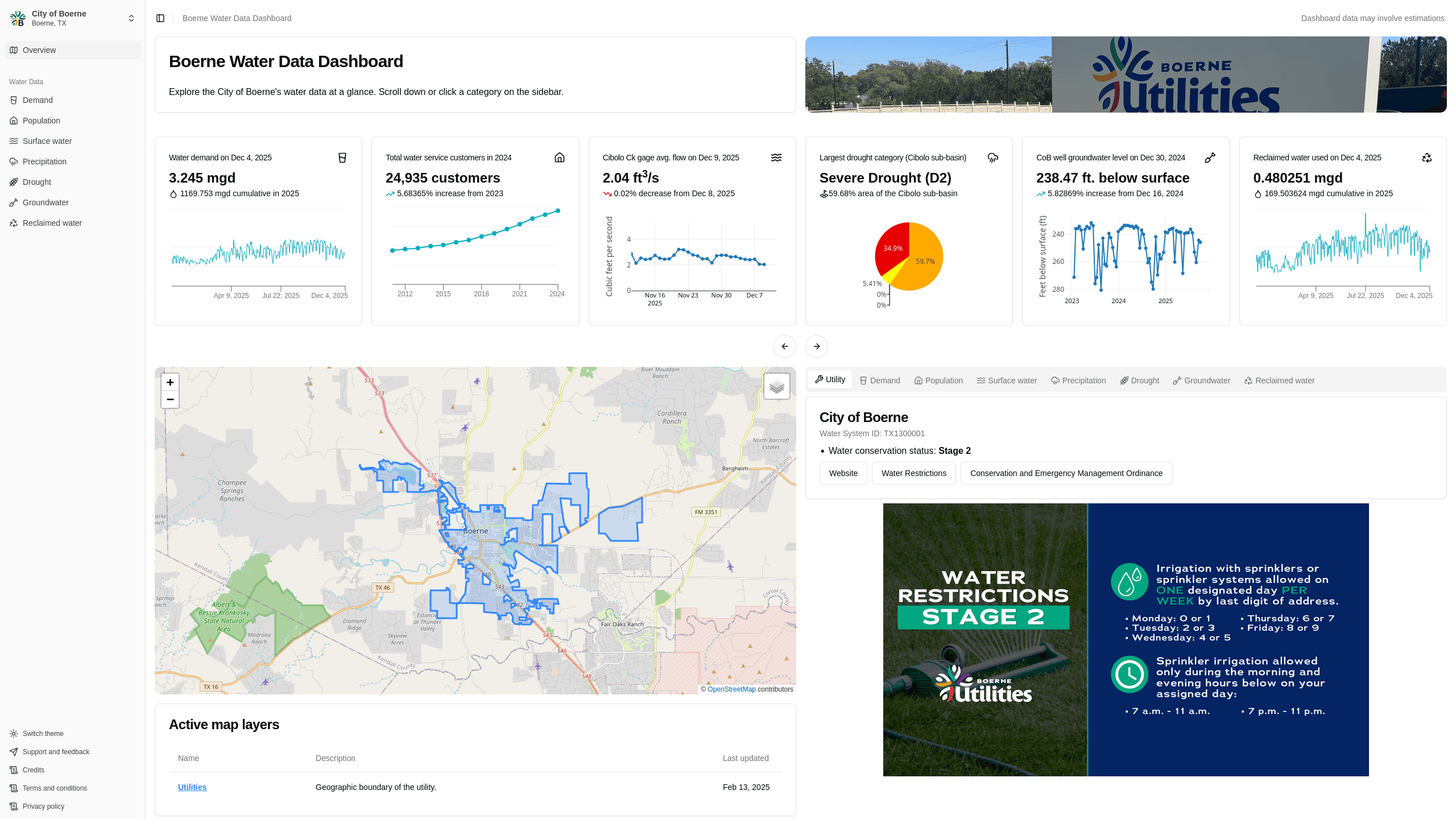
Boerne Water Data Dashboard
Next.js
Rust
Data visualization
Data engineering
Polars
Plotly
commit-helper
Rust
Building a CKAN Release Timeline

Python
CKAN
TimelineJS v3
HTML
View more written content on my blog.